3 strong examples for understanding Machine Learning and Naive Bayes

In today’s article, we will discuss artificial intelligence, specifically the concept of machine learning. Artificial intelligence, or AI, refers to methods that simulate human behavior or imitate human intelligence in order to perform tasks that can be improved iteratively over time as new information is accumulated.

However, what exactly is machine learning?

The historical context:

A brief historical overview of this concept dates back to the 1930s. Alan Turing, a famous mathematician and cryptologist who was responsible for the decipherment of the Enigma machine during the World War II, created the concept of the “universal machine” (Turing, 1936)¹. This machine is the basis for today’s computers. Also during this period, an article describing the functioning of neurons with the assistance of electrical circuits served as the theoretical basis for work on neural networks (McCulloch & Pitts, 1943)². Arthur Samuel was the first researcher to theorize the concept of machine learning. His research demonstrated how his checkers program improved as it played (Samuel, 1959)³.

An overview of machine learning:

Our earlier introduction explained that artificial intelligence is a concept that simulates human behavior. Essentially, machine learning can be defined as the process of achieving artificial intelligence. We can use Arthur Samuel’s checkers game as an example to illustrate what machine learning is. As a result, he attempted to make his program learn from his mistakes in order to strengthen itself and avoid making the same mistakes again. In this regard, we may define machine learning as the ability of a machine to learn without being explicitly programmed to do so. As a result, it would accumulate data in order to become more accurate and less prone to making errors as a result.

Overview of different machine learning methods:

They all relate to statistical prediction models, which can be used to resolve one or more problems. Let us now examine the mechanism of the machine in order to better understand how it operates.

The process:

This video provides a good description of machine learning:

https://www.youtube.com/watch?v=SX08NT55YhA

An example is provided here of how a machine learns from its mistakes and progresses through the use of reward systems and punishment systems when mistakes are made. The device is able to self-correct and learn from its mistakes with this amount of input. However, as shown in the video, there is the risk of overfitting.

Generally, overfitting refers to a model that has been overtrained or overadjusted. In other words, if we take the example of the car that learns to drive in the game, it only knows how to do so in accordance with what it has already learned. As a result, it is unable to respond appropriately to different patterns (in this case, straight lines). A model that has been overfitted can only be used for its own datasets, and cannot be applied to other datasets due to the overfitting. To prevent overfitting, a number of methods are available, including data simplification, data assembling, and cross-validation. Based on the example of the video, the car learns on other parts of the track in order to perfect its learning model. Furthermore, it is exposed to a variety of situations during its course of operation.

If we position the car in other parts of the circuit in the example, it will behave as it did at the beginning by learning the new parts of the circuit. As a result of this learning of new elements, the car can now move across a longer section of the circuit when it is put back at the beginning, since it has recognized the new patterns it has previously learned. Our algorithm has been trained, and it will now be put to the test on the track.

However, as the example presented indicates, there are some difficulties. It takes the car much longer to complete the circuit than it does for a human, due to the complexity of the track in the example. Additionally, as demonstrated in the video example, the AI could be beaten by skilled players, but probably not by novice players.

This video example illustrates both the strengths and weaknesses of machine learning. Artificial intelligence is capable of learning how to turn and move on circuits, which is a significant strength. Despite its rapid evolution, it is unable to evolve further due to problems associated with overfitting. By applying different methods, the machine will be able to evolve and solve problems it may encounter in the future.

Why is it used?

There are dozens of possible predictive algorithms in machine learning, as previously discussed. Depending on the initial problem, these models represent different solutions. Additionally, different types of algorithms can be applied to solve a given problem, which makes the task complex if it is not understood which algorithm to apply. By using an example, we will illustrate how the Bayesian model can be implemented and its usefulness.

A Bayesian statistical model

As part of its foundation, this statistical model is based on the probability of seeing a particular event in light of existing conditions that are likely to be related to that event. In other words, if the risk of developing health problems increases with age (WHO)⁵, Bayes’ theorem provides a more accurate assessment of the risk to an individual of a known age (by conditioning it on their age) than simply assuming that the individual is typical of the entire population.

Formula:

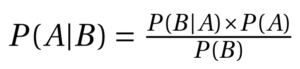
= Probability a hypothesis is true given some evidence

= Probability of seeing the evidence if the hypothesis is true

= Probability a hypothesis is true before any evidence

= Probability of seeing the evidence

A case study of Steve

A neighbour described the individual as follows: “Steve is very shy and withdrawn, invariably helpful but with little interest in people or in the world of reality. A meek and tidy soul, he has a need for order and structure, and a passion for detail.”

A study conducted by Tversky and Kahneman (1974)⁴ addressed the following question:

Would Steve be more likely to be a librarian or a farmer?

 

It would be reasonable to assume that the librarian would be in the majority, since he is described as being “meek and tidy“. As a result, we are reinforced in our stereotypes and beliefs about the individual, leading us to refer to him as a librarian rather than as a farmer. According to the example, 90% of respondents identify him as a librarian, while only 10% identify him as a farmer.

To better understand this, it is helpful to know the proportion of farmers to librarians in a given country. It is estimated that there is one librarian for every 20 farmers in this example.

Let us return to the example and suppose that 40% of librarians and 10% of farmers fit this description. There are 4 librarians out of 10 and 20 farmers out of 200 (remember that the ratio is 1 librarian to 20 farmers).

By replacing the terms in the formula, we observe that it is estimated that the

P(Librarian given the description) will be

4/(4+20)≈16.7%

As a matter of fact, your belief has changed here. Check out this video that explains the Bayes Theorem in a much more thorough manner with the same example as Steve’s:

https://www.youtube.com/watch?v=HZGCoVF3YvM

Support for decision-making

As last example on this article, we will demonstrate how Naive Bayes can be used to solve the problem of spam that we all receive in our inboxes. We are attempting to assign probabilities to words in classic emails that we receive in order to categorize them as “normal“. Then, we apply the same principle to the words used in the “spam” email messages. As a part of the training process, the algorithm is trained to recognize the most frequently used words in spam messages compared to the most commonly used words in normal messages. As a result of this analysis, we are able to generate probabilities associated with being recognized as “normal” or “spam“. In addition, we assess the probability that certain messages are more associated with normal mail than spam when they are included in a message. As a result, we categorize messages as “normal” or “spam” in our mailboxes.

By using Bayes’ statistical model for example, the entire decision-making process is based on statistics and therefore on the probability of belonging to a particular group. The video can be viewed here for a more detailed explanation of how it works using the example of e-mails.

https://www.youtube.com/watch?v=O2L2Uv9pdDA

Additionally, the following resources can provide you with additional information on Bayesian networks:

https://medium.com/eliiza-ai/bayesian-networks-combining-machine-learning-and-expert-knowledge-into-explainable-ai-efaf6f8e69b

References

1. Turing, A. M. (1936). On computable numbers, with an application to the Entscheidungsproblem. J. of Math, 58(345-363), 5.
2. McCulloch, W. A. S., and Pitts, W. (1943). A Logical Calculus of the Ideas Immanent in Nervous Activity, Bulletin of Mathematical Biology 5, 115-133.
3. Samuel, A. L. (1959). Machine learning. The Technology Review, 62(1), 42-45.
4. Tversky, A., & Kahneman, D. (1974). Judgment under Uncertainty: Heuristics and Biases: Biases in judgments reveal some heuristics of thinking under uncertainty. science, 185(4157), 1124-1131.
5. https://www.who.int/news-room/fact-sheets/detail/ageing-and-health